Chapter 4 Missing values

4.1 Disaster dataset

disaster = read.csv("data/disaster_missing.csv") %>%
  select(-X)

4.1.1 By row

rowSums(is.na(disaster)) %>%
  sort(decreasing = TRUE) %>%
  table()

## .
##     0     1     2     3     4 
##  3555  1748 14669  4781   742

It shows that the missing value numbers with different rows. There are for 3555 rows with no missing values, 1748 rows with 1 missing values, 14669 rows with 2 missing values, 4781 rows with 3 missing values and 742 rows with 4 missing values.

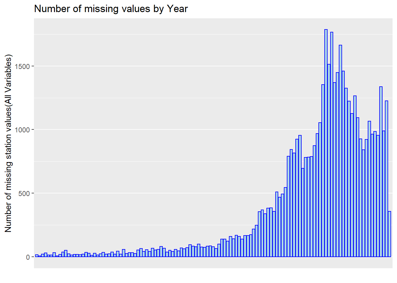
Also we want to visualize it by year.

missing <- disaster %>% 
    group_by(Year) %>% 
    summarise(sum.na = sum(is.na(Total.Deaths)+is.na(Total.Damages)+is.na(Disaster.Subtype)+is.na(Total.Damages.Adjusted)))

ggplot(missing, aes(x = Year, y = sum.na)) +
  geom_col(color = "blue", fill = "lightblue") +
  ggtitle("Number of missing values by Year") +
  xlab("") +
  ylab("Number of missing station values(All Variables)") +
  theme(axis.text.x = element_text(angle = 45)) +
  scale_x_discrete(breaks = c('1900','1910','1920','1930','1940','1950','1960','1970','1980','1990','2000','2010','2020'))

It shows that the missing value has a increasing trend among all years because the data records are increasing over year.

4.1.2 By Column

colSums(is.na(disaster)) %>%
  sort(decreasing = TRUE)

## Total.Damages.Adjusted          Total.Damages           Total.Deaths 
##                  19931                  19917                   5334 
##       Disaster.Subtype                   Year         Disaster.Group 
##                   3215                      0                      0 
##      Disaster.Subgroup          Disaster.Type                Country 
##                      0                      0                      0 
##                    ISO                 Region              Continent 
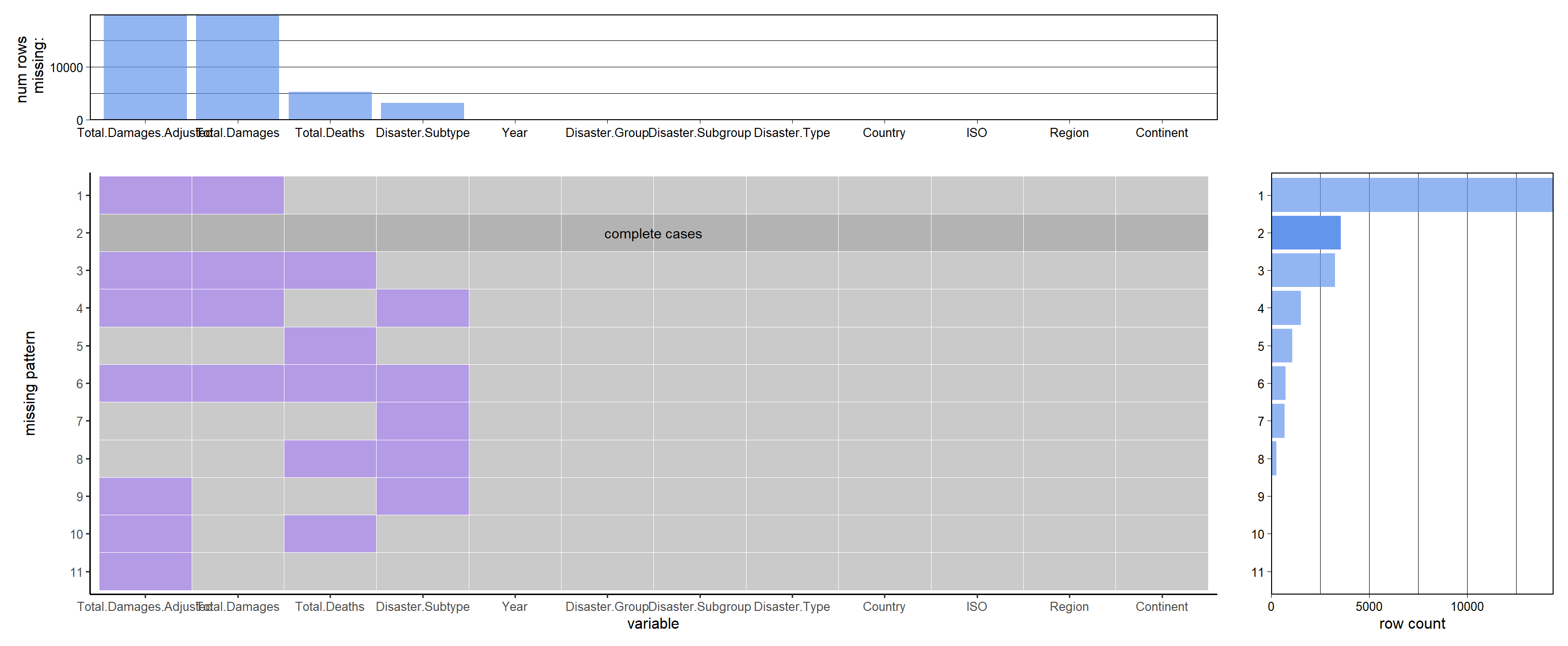
##                      0                      0                      0

plot_missing(disaster, percent = FALSE)

It shows that damage and adj.damage gets the most nas, then deaths and subtype.

4.1.3 By Value

tidydata <- disaster %>% 
    rownames_to_column("id") %>% 
    gather(key, value, -id) %>% 
    mutate(missing = ifelse(is.na(value), "yes", "no"))

ggplot(tidydata, aes(x = key, y = fct_rev(id), fill = missing)) +
  geom_tile() + 
  ggtitle("ourdata with NAs") +
  scale_fill_viridis_d() + # discrete scale
  theme_bw()+
  scale_y_discrete(breaks = c())

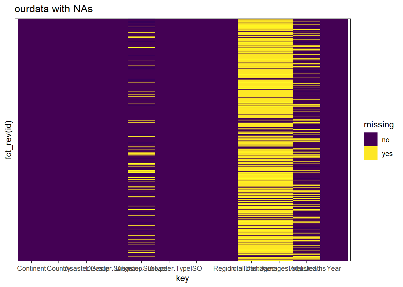
It gives a look at the na for each value. However I don’t think that there is a relation between the nas in different variable.

4.2 Covid Dataset

covid = read.csv("data/covid.csv") %>%
  select(-X)

sum(is.na(covid))

## [1] 0

There is no NA value in this data set.

4.3 GDP Dataset

GDP = read.csv("data/GDP.csv")

This is a time series data from 1960 to 2020 for the countries around the world, we want to check the na for each countries and for each Year.

4.3.1 For countries

We want to see how many NA are there for each country

missing = cbind(GDP[,1:2], NAs = rowSums(matrix(as.numeric(is.na(GDP[,-c(1,2)])), nrow = nrow(GDP)))) %>%
  arrange(desc(NAs))

head(missing, 10)

##      X               Country.Name NAs
## 1   28     British Virgin Islands  61
## 2   76                  Gibraltar  61
## 3  104                North Korea  61
## 4  184 Saint Martin (French part)  61
## 5  173               Sint Maarten  53
## 6  179                South Sudan  53
## 7   40            Channel Islands  51
## 8   51                   CuraÃ§ao  51
## 9  138                      Nauru  50
## 10 106                     Kosovo  48

As we can see, the missing value are tend to appear on those small countries where data are hard to collect.

4.3.2 For Year

Now we want to know the missing value among time

missing = cbind(Year = 1960:2020, NAs = colSums(matrix(as.numeric(is.na(GDP[,-c(1,2)])), nrow = nrow(GDP))))

## Warning in cbind(Year = 1960:2020, NAs = colSums(matrix(as.numeric(is.na(GDP[, :
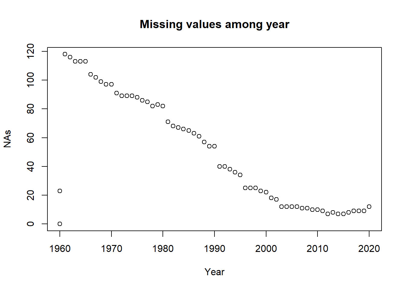
## number of rows of result is not a multiple of vector length (arg 1)

plot(missing, main = 'Missing values among year')

Here as we can see, the missing values are reducing with the year increase. That’s because with the development of the technology, we have more and easier access to collect the data.